Scanning Tunneling Microscopy

The basic geometry

Fig. 1 Schematic of STM tip and sample.

The scanning tunneling microscope was invented in 1982 by Binnig and Rohrer, for which they shared the 1986 Nobel Prize in Physics. The instrument consists of a sharp conducting tip which is scanned across a flat conducting sample. When a bias voltage V_b is applied between tip and sample, a current will flow, and this current can be measured as a function of (x, y) location and as a function of V_b. This is illustrated schematically in Figure 1.

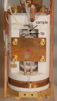
Fig. 2 Photograph of STM.

A photograph of an STM built in the Hoffman Lab is shown in Figure 2. Here, the tip is pointing upwards, and the sample is inserted face-down from above. The tip is attached to the end of a 4-quadrant scan piezo, i.e. a cylindrical piece of ceramic which bends (and scans the tip) according to the voltages applied to the four quadrants.

This STM is operated in vacuum, typically at 4.2 K, the boiling temperature of liquid helium. Because the walls of the vacuum chamber are so cold, any unwanted gas molecule which may be bouncing around in the vacuum chamber will stick to the first wall it hits. This means that the vacuum is very good indeed, typically less than 10^-13 Torr (that's about 10^-16 times atmospheric pressure!) This vacuum is very important, because we do not want rogue oxygen or water molecules sitting on the nice clean sample surface we are trying to study.

So what is this tunneling current anyhow?

In order to understand the tunneling current, first we have to talk about "density of states". Electrons in an isolated atom live at specific discrete energy levels. Likewise in a metal, the electrons must live at specific energy levels, based on the energy landscape of the metal. The difference is, that in a macroscopic piece of metal there are so many electrons that the energy level spacing gets very close together. The levels are so close together that it no longer makes sense to try to list the energy levels of all the electrons. (There are 10²³ electrons in a macroscopic piece of metal, so it would actually take us 10¹⁶ years, that's 6 million times the age of the universe, to write down all the energy levels at a rate of one per second!) So, instead we ask the question, in a given energy interval Δε around energy ε, how many electrons are there?

tunneling smileys

Fig. 3: The electrons fill up the energy valley in the sample until there are no more electrons. The top energy level at which electrons sit is called the Fermi level, ε_F. For every energy ε, the density of states is the number of electrons sitting within Δε of ε, divided by Δε. So, for the energy shown above as a blue strip, DOS(ε) is approximately 7 / Δε.

Another relevant question is, why do the electrons all sit on top of each other, filling up the valley to energy ε? Why wouldn't they all just clump together at the lowest point at the bottom of the valley? The answer is that electrons are rather unfriendly characters called fermions. No two fermions are allowed to occupy the same energy state; this is known as the Pauli exclusion principle. So the electrons must pile on top of each other instead.

Electrons are happy sitting in either the tip or the sample, i.e. they're sitting in nice energy valleys. But it takes energy to remove an electron into free space. We can think of the vacuum around the tip as an energy hill that the electron would need to climb in order to escape. The height of this energy hill is called the work function, φ.

tunneling smileys

Fig. 4: The electrons in the tip and the sample are sitting in two separate valleys, separated by a hill which is the vacuum barrier.

In order to bring an electron up and over the vacuum energy barrier from the tip into the sample (or vice versa), we would need to supply a very large amount of energy. Climbing hills is hard work! Luckily for us, quantum mechanics tells us that the electron can tunnel right through the barrier. Note: this only works for particles, not for macroscopic objects. Don't you try walking through any closed doors!

OK, great, so the electrons can tunnel and we can measure the tunneling current. But not so fast, we need to remember the Pauli exclusion principle. Even if the electrons in Fig. 4 can tunnel through the energy barrier, they have no place to go. As long as both the tip and the sample are held at the same electrical potential, their Fermi levels line up exactly. There are no empty states on either side available for tunneling into! This is why we apply a bias voltage between the tip and the sample.

tunneling smileys

Fig. 5: By applying a bias voltage to the sample with respect to the tip, we effectively raise the Fermi level of the sample with respect to the tip. Now we have empty states available for tunneling into.

The current which flows between the tip and the sample depends on the voltage difference between the tip and sample. If the sample is biased by a negative voltage -V with respect to the tip, this effectively raises the energy level of the sample electrons with respect to the tip electrons by an energy eV. Electrons will tend to tunnel out of the filled states of the sample, into the empty states of the tip.

The total tunneling current will be proportional to the number of filled states on the left available for tunneling from, times the number of empty states on the right available for tunneling to. In other words, the tunneling current is proportional to the integral of the density of states of the sample, up to some energy eV. By varying the bias voltage V, we can therefore map out the density of states of the sample, DOS(ε).

[More technical explanation of STM]